PySAP Basics

Code author: Antoine Grigis <antoine.grigis@cea.fr>

This example introduces some of the basic features of the core PySAP package as well as some tests to ensure that everything has been installed correctly.

First checks

In order to test if the pysap package is properly installed on your machine, you can check the package version.

import matplotlib.pyplot as plt
import pysap

print(pysap.__version__)

Out:

0.2.1

Now you can run the the configuration info function to see if all the dependencies are installed properly:

import pysap.configure

print(pysap.configure.info())

Out:

                 .|'''|       /.\      '||'''|,
                 ||          // \\      ||   ||
'||''|, '||  ||` `|'''|,    //...\\     ||...|'
 ||  ||  `|..||   .   ||   //     \\    ||
 ||..|'      ||   |...|' .//       \\. .||
 ||       ,  |'
.||        ''

Package version: 0.2.1

License: CeCILL-B

Authors:
The PySAP Team
Dependencies:

scipy          : >=1.5.4   - required | 1.11.4    installed
numpy          : >=1.19.5  - required | 1.26.3    installed
matplotlib     : >=3.3.4   - required | 3.8.2     installed
astropy        : >=4.1     - required | 6.0.0     installed
nibabel        : >=3.2.1   - required | 5.2.0     installed
progressbar2   : >=3.53.1  - required | ?         installed
modopt         : >=1.6.1   - required | 1.7.1     installed
scikit-learn   : >=0.24.1  - required | ?         installed
scikit-image   : >=0.17.2  - required | ?         installed
pywt           : >=1.1.1   - required | 1.5.0     installed
pysparse       : >=0.0.1   - required | 0.1.0     installed

Import astronomical data

PySAP provides a common interface for importing and visualising astronomical FITS datasets. A sample of toy datasets is provided that will be used in this tutorial.

import pysap
from pprint import pprint
from pysap.data import get_sample_data

image = get_sample_data('astro-fits')
print(image.shape, image.spacing, image.data_type)
pprint(image.metadata)
print(image.data.dtype)
plt.imshow(image)
plt.show()

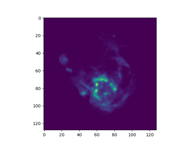
Out:

(128, 128) [1. 1.] scalar
{'BITPIX': -64,
 'COMMENT': "  and Astrophysics', volume 376, page 359; bibcode: "
            '2001A&A...376..359H',
 'EXTEND': True,
 'NAXIS': 2,
 'NAXIS1': 128,
 'NAXIS2': 128,
 'SIMPLE': True,
 'path': '/home/cg260486/.local/share/pysap/M31_128.fits'}
float32
/volatile/Chaithya/actions-runner/_work/pysap/pysap/examples/pysap/plot_basics.py:48: UserWarning: FigureCanvasAgg is non-interactive, and thus cannot be shown
  plt.show()

Import neuroimaging data

PySAP also provides a common interface for importing and visualising neuroimaging NIFTI datasets. A sample of toy datasets is provided that will be used in this tutorial.

import pysap
from pprint import pprint
from pysap.data import get_sample_data

image = get_sample_data('mri-nifti')
image.scroll_axis = 2
print(image.shape, image.spacing, image.data_type)
pprint(image.metadata)
print(image.data.dtype)
# image.show()  ## uncomment to visualise this object

Out:

(240, 256, 160) [1.  1.  1.1] scalar
{'path': '/home/cg260486/.local/share/pysap/t1_localizer.nii.gz'}
float32

Decompose/recompose an image using a fast Sparse2D based transform

PySAP includes Python bindings for the Sparse2D C++ library of wavelet transforms developped at the CosmoStat lab. PySAP also uses the PyWavelet package. The code is optimsed and provides access to many image decompsition strategies.

All the transforms available can be listed as follows.

from pprint import pprint
import pysap

pprint(pysap.wavelist())
pprint(pysap.wavelist(family='isap-3d'))

Out:

{'isap-2d': ['BsplineWaveletTransformATrousAlgorithm',
             'DecompositionOnScalingFunction',
             'FastCurveletTransform',
             'FeauveauWaveletTransform',
             'FeauveauWaveletTransformWithoutUndersampling',
             'HaarWaveletTransform',
             'HalfPyramidalTransform',
             'IsotropicAndCompactSupportWaveletInFourierSpace',
             'LineColumnWaveletTransform1D1D',
             'LinearWaveletTransformATrousAlgorithm',
             'MallatWaveletTransform79Filters',
             'MeyerWaveletsCompactInFourierSpace',
             'MixedHalfPyramidalWTAndMedianMethod',
             'MixedWTAndPMTMethod',
             'MorphologicalMedianTransform',
             'MorphologicalMinmaxTransform',
             'MorphologicalPyramidalMinmaxTransform',
             'NonOrthogonalUndecimatedTransform',
             'OnLine44AndOnColumn53',
             'OnLine53AndOnColumn44',
             'PyramidalBsplineWaveletTransform',
             'PyramidalLaplacian',
             'PyramidalLinearWaveletTransform',
             'PyramidalMedianTransform',
             'PyramidalWaveletTransformInFourierSpaceAlgo1',
             'PyramidalWaveletTransformInFourierSpaceAlgo2',
             'UndecimatedBiOrthogonalTransform',
             'UndecimatedDiadicWaveletTransform',
             'UndecimatedHaarTransformATrousAlgorithm',
             'WaveletTransformInFourierSpace',
             'WaveletTransformViaLiftingScheme'],
 'isap-3d': ['ATrou3D',
             'BiOrthogonalTransform3D',
             'Wavelet3DTransformViaLiftingScheme'],
 'pywt': ['bior11',
          'bior13',
          'bior15',
          'bior22',
          'bior24',
          'bior26',
          'bior28',
          'bior31',
          'bior33',
          'bior35',
          'bior37',
          'bior39',
          'bior44',
          'bior55',
          'bior68',
          'cgau1',
          'cgau2',
          'cgau3',
          'cgau4',
          'cgau5',
          'cgau6',
          'cgau7',
          'cgau8',
          'cmor',
          'coif1',
          'coif10',
          'coif11',
          'coif12',
          'coif13',
          'coif14',
          'coif15',
          'coif16',
          'coif17',
          'coif2',
          'coif3',
          'coif4',
          'coif5',
          'coif6',
          'coif7',
          'coif8',
          'coif9',
          'db1',
          'db10',
          'db11',
          'db12',
          'db13',
          'db14',
          'db15',
          'db16',
          'db17',
          'db18',
          'db19',
          'db2',
          'db20',
          'db21',
          'db22',
          'db23',
          'db24',
          'db25',
          'db26',
          'db27',
          'db28',
          'db29',
          'db3',
          'db30',
          'db31',
          'db32',
          'db33',
          'db34',
          'db35',
          'db36',
          'db37',
          'db38',
          'db4',
          'db5',
          'db6',
          'db7',
          'db8',
          'db9',
          'dmey',
          'fbsp',
          'gaus1',
          'gaus2',
          'gaus3',
          'gaus4',
          'gaus5',
          'gaus6',
          'gaus7',
          'gaus8',
          'haar',
          'mexh',
          'morl',
          'rbio11',
          'rbio13',
          'rbio15',
          'rbio22',
          'rbio24',
          'rbio26',
          'rbio28',
          'rbio31',
          'rbio33',
          'rbio35',
          'rbio37',
          'rbio39',
          'rbio44',
          'rbio55',
          'rbio68',
          'shan',
          'sym10',
          'sym11',
          'sym12',
          'sym13',
          'sym14',
          'sym15',
          'sym16',
          'sym17',
          'sym18',
          'sym19',
          'sym2',
          'sym20',
          'sym3',
          'sym4',
          'sym5',
          'sym6',
          'sym7',
          'sym8',
          'sym9']}
{'isap-3d': ['ATrou3D',
             'BiOrthogonalTransform3D',
             'Wavelet3DTransformViaLiftingScheme']}

Here we illustrate the the decomposition/recomposition process using a Daubechies ('db3') wavelet from pywt with 4 scales:

import pysap
from pysap.data import get_sample_data

image = get_sample_data('mri-slice-nifti')
transform_klass = pysap.load_transform('db3')
transform = transform_klass(nb_scale=4, verbose=1, padding_mode='symmetric')
transform.data = image
transform.analysis()
# transform.show()  ## uncomment to visualise this object
rec_image = transform.synthesis()
# rec_image.show()  ## uncomment to visualise this object

Here we illustrate the the decomposition/recomposition process using a fast curvelet transform ('FastCurveletTransform') from Sparse2D with 4 scales:

image = get_sample_data('mri-slice-nifti')
transform_klass = pysap.load_transform('FastCurveletTransform')
transform = transform_klass(nb_scale=4, verbose=1, padding_mode='zero')
transform.data = image
transform.analysis()
# transform.show()  ## uncomment to visualise this object
rec_image = transform.synthesis()
# rec_image.show()  ## uncomment to visualise this object